Implementation
Here, we describe the implementation details of Undefined on how we achieve the automatic differentiation.
5.1 Core Data Structure
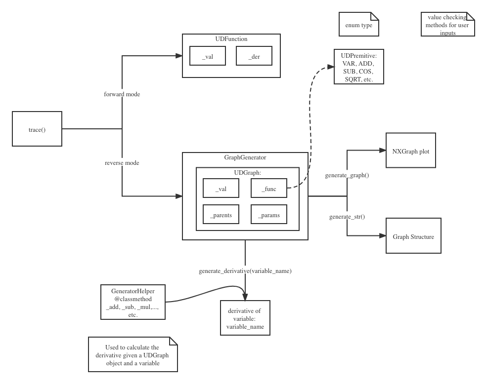
Here is the general workflow in our main function and how they connect with other .py files. The two main branches in the implementation are the “forward mode” and “reverse mode”. We will discuss in details below.
Forward Mode
To calculate the derivative in forward mode, we used the dual number approach. In the `UDFunction` class inside the UDFunction.py, we overloaded the operators and accommodated the dual number (as the core data structure) approach following the formula below:
\({z}_j = {v}_j + D_p v_j \epsilon\)
where \({v}_j\) is the real part corresponding to the primal trace, and the \({D_p v_j}\) is the dual part corresponding to the tangent trace.
5.2 Extension Implementation
Reverse Mode
The reverse mode calculates the partial derivatives of the i-th output \(f_i\) with respect to the n variables \(v_{j-m} = x_j\) with j = 1,2,…,n by traversing the computational graph backwards. The partial derivatives describe the _sensitivity_ of the output with respect to the intermediate variable \(v_{j-m}\):
\(\bar v_{j-m} = \frac{\partial f_i}{\partial v_{j-m}}\)
The two steps approach we utilized are Forward pass and Reverse pass
Forward pass
In the forward pass, we compute the primal value \(v_j\) and the partial derivatives \(\frac{\partial v_j}{\partial v_i}\) with respect to its parent nodes \(v_i\). This partial derivatives here are the factors that show up in the chain rule, but it’s not the chain rule itself. Given the unique way of the implementation in reverse mode, we are not explicitly calculating the chain rule in the forward pass, but calculate it as we build up the computational graph.
For example, in the forward pass, given the function \(v_j = sin(v_j)\), we calculate \(\frac{\partial v_j}{\partial v_i} = cos(v_i)\).
In the reverse model, we implemented a graph structure (UDGraph) to store the parent and child intermediate results.
Reverse pass
In the reverse pass, we reconstruct the chain rule that we ignored in the forward pass. The goal is to compute each node of \(v_i\):
\(v_i = \frac{\partial f}{\partial v_i} = \sum_{j\ a\ child\ of\ i} \frac{\partial f}{\partial v_j} \frac{\partial v_j}{\partial v_i} = \sum_{j\ a\ child\ of\ i} v_j \frac{\partial v_j}{\partial v_i}\)
The \(\frac{\partial v_j}{\partial v_i}\) was calculated during the forward pass, so in the reverse pass, we just need to initialize \(v_i = 0\) and update the values as we iterate over each parental and child node with the following equation:
\(v_i = v_i + \frac{\partial f}{\partial v_j} \frac{\partial v_j}{\partial v_i} = v_i + v_j \frac{\partial v_j}{\partial v_i}\)
Lastly, once we reached to the last intermediate step, we will have \(v_{n-m} = f(x)\) with \(x \in \mathbb{R}\) and this last node do not have children. To deal with this, we know the initial value of the adjoint \(v_{n-m]\):
\(v_{n-m} = \frac{\partial f}{\partial v_{n-m}} = \frac{\partial v_{n-m}}{\partial v_{n-m}} = 1\)
which we need to get started as in the reverse pass we traverse the computational graph backwards, from the right, which is the outputs to the left (the input).
In the reverse mode, we used the UDPremitive class serving as a look up table to help us to calculate the derivative in the reverse mode.
One thing to note is that mathematically, we only work with numerical values, not with formulae or overladed operators. However, to automatically build the computational graph structure, we modified the operators for the reverse mode so that we can save the intermediate values as we do the calculation.
This is implemented in the GraphGenerator.py file.
5.3 Core Classes
We used numpy and math libraries to help with the math and used matplotlib and networkx libraries for plot the computational graph.
The methods and descriptions below are only included the major functions. Helper functions are not included. Please refer to the source code for all detailed function description.
API.py: This class contains methods that can be called by the users, the trace function. Here is the default setting for the trace function. The default mode is the “forward” mode, the default seeds = None, and plot = False.
1trace(lambda_function, mode="forward", seeds = None, plot=False, **kwargs)
UDFunction.py:
This class wraps the core data structure in our library. Objects instantiated from this class are the most basic computing units in our library.
Name Attributes:
Name Attribute |
Description |
|---|---|
values |
values of a elementary function |
derivatives |
derivatives of a elementary function |
shape |
a tuple that declares the shape of values attribute |
Methods:
In this file, we overloaded all the Dunder/Magic Methods and the comparison methods in Python, including the following:
__add__ and __radd__
__sub__ and __rsub__
__mul__ and __rmul__
__sub__ and __rsub__
__truediv__ and __rtruediv__
__floordiv__ and __rfloordiv__
__pow__ and __rpow__
__neg__
__eg__ and __ne__
__lt__ and __gt__
__le__ and __ge__
Calculator.py:
This class contains functions to perform elementary functions calculation on UDFunction such as sin, sqrt, log, exp, which cannot be implemented by overloaded functions in UDFunction.
Method |
Description |
|---|---|
cos(udobject) |
calculate cos value of a udobject |
sin(udobject) |
calculate sin value of a udobject |
tan(udobject) |
is calculated tan by using sin(udobject) and cos(udobject) |
sqrt(udobject) |
square root performed on udobject |
exp(udobject) |
exponential performed on udobject |
log(udobject, base=numpy.e) |
logarithms of base: base. Default base is np.e. |
standard_logistic(udobject) |
standard logistic |
One thing to note for log is that we do not support other log functions from other library, such as np.log2().
In that case, you will need to do log(user_defined_function, 2) for our program to work.
Moreover, we also have extended our math operations to inverse trig functions.
Method |
Description |
|---|---|
sinh(udobject) |
calculate sinh value of a udobject |
cosh(udobject) |
calculate cosh value of a udobject |
tanh(udobject) |
calculate tanh value of a udobject |
coth(udobject) |
calculate coth value of a udobject |
sech(udobject) |
calculate sech value of a udobject |
csch(udobject) |
calculate csch value of a udobject |
arccos(udobject) |
calculate arccos value of a udobject |
arcsin(udobject) |
calculate arcsin value of a udobject |
arctan(udobject) |
calculate arctan value of a udobject |
GraphGenerator.py:
For the reverse mode, we defined our class named UDGraph. In this class, we modified the Dunder/Magic methods mentioned above so that it will start building the computational graph structure spontaneously as the computation goes.
The methods included in this class are:
__add__ and __radd__
__sub__ and __rsub__
__mul__ and __rmul__
__sub__ and __rsub__
__truediv__ and __rtruediv__
__floordiv__ and __rfloordiv__
__pow__ and __rpow__
__neg__
__eg__ and __ne__
__lt__ and __gt__
__le__ and __ge__
To achieve building the graph structure, we also created a class called GeneratorHelper class to help build the graph structure.
Another class we developed in this file is the GraphGenerator, which will facilitate generating the output figure and the print out the graph structure as outputs. Refer to the reverse mode demo section.
Utils.py:
We defined our Enum type of class here, the UDPrimitive.
5.4 External Dependencies
Both TravisCI and CodeCov are used for testing suit monitoring. The CI status and the code coverage are reflected in our github repository. The package have been uploaded and distributed via PyPI . We used the NetworkX package for constructing the visualization for the computational graph.
Lastly, we used the numpy and math libraries to help with the math calculation.