About
1. Introduction
Automatic Differentiation (AD) refers to the way to compute the derivative of a given equation automatically. It has a broad range of applications across many disciplines, such as engineering, statistics, computer science, and computational biology. For both students and researchers, it is essential for them to have tools in order to compute derivatives efficiently, given the amount of computational power needed. Here, we propose a novel Python library, undefined, to implement the AD on user defined numerical equations.
One potential application would be calculating the derivatives in the direction of negative gradient to minimize the loss function when tuning parameters in training gradient machine learning models. Undefined is easier to use, single task focused, and efficient.
2. Background
As we learned in calculus classes, the traditional way to calculate derivatives is to calculate by hand and apply different rules, including power rule, product rule, chain rule, etc.
Here is an example when we need to calculate a derivative by using the chain rule.
2.1 Chain Rule Formula
The general formula of the chain rule is shown as following:
Suppose we have a function \(h(u(t))\), then the derivative of this function would be shown as the following:
\(\frac{dh}{dt} = \frac{\partial h}{\partial u}\frac{du}{dt}\)
When we have multiple coordinates, the chain rule formula will change:
Suppose our formula is \(h(u(t), v(t))\), then the derivative of this function would be shown as the following:
\(\frac{dh}{dt} = \frac{\partial h}{\partial u}\frac{du}{dt} + \frac{\partial h}{\partial v}\frac{dv}{dt}\)
2.2 Elementary Function
Unary elementary function examples:
sin(x),cos(x)Binary elementary function examples:
x + y,x * y
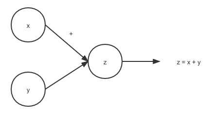
2.3 Computational Graph
A computational graph is a directed graph where the nodes correspond to elementary functions or variables.
Computational graph node for binary elementary function:
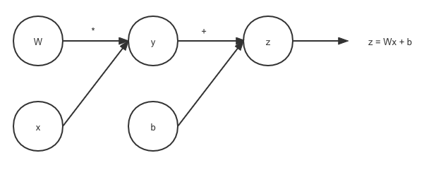
The computational graph grows once the computations become more complex:
2.4 Automatic Differentiation
Suppose we have the gradients of the function defined as following:
\(f(x, y) = \cos(5x + 7y)e^{-x}\)
Assume we will calculate the partial derivative for x first, \(\frac{\partial f}{\partial x}\), we will apply the product rule first:
\(\frac{\partial f}{\partial x} = \cos(5x + 7y)(-e^{-x}) - 5 \sin(5x + 7y)e^{-x}\)
To simplify:
\(\frac{\partial f}{\partial x} = -e^{-x}(\cos(5x+7y) + 5\sin(5x+7y))\)
If we would have to calculate \(\frac{\partial f}{\partial y}\), we only need to use the chain rule:
\(\frac{\partial f}{\partial y} = -7\sin(5x + 7y)e^{-x}\)
Computing this function is simple, but AD will become handy when we have to compute the derivative for complicated equations.
There are many advantages of AD compared to traditional methods such as numerical differentiation and symbolic differentiation. One of the most signifigant advantages of AD is that it calculates to machine precision while preserving accuracy and stability.
Here, we provided two different ways to calculate the derivative automatically, the forward and the reverse modes.
Generally speaking, one of the key elements in the forward mode is the Jacobian matrix \(J = \frac{\partial f_i}{\partial x_j}\), which is a matrix containing the partial derivatives of all the outputs with respect to all the inputs.
If \(f\) has a one-dimensional output, the Jacobian matrix is just the gradient. The solution of systems of equations requires differentiation of a vector-function of multiple variables.
Later in the implementation section, you will see how you can change seed from the Jacobian matrix so that you can control which derivative you want to take.
The equations and motivations of using AD are inspired by CS107/AC207 lecture materials.